

The bias-variance tradeoff is a fundamental concept in machine learning that deals with the tradeoff between the bias of a model and its variance. It’s crucial for understanding the behavior of machine learning algorithms and for building models that generalize well to unseen data.
Bias
Bias refers to the error introduced by approximating a real-world problem with a simplified model. A high bias model makes strong assumptions about the underlying data and is typically oversimplified. It tends to underfit the data, meaning it fails to capture the true relationships present in the data. Models with high bias have low complexity and may perform poorly on both the training and test datasets.
Variance
Variance refers to the amount by which a model’s prediction would change if trained on a different dataset. High variance models are overly complex and tend to capture noise in the training data. They perform well on the training data but poorly on unseen data because they fail to generalize. High variance models are prone to overfitting.
Tradeoff
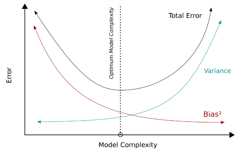
The bias-variance tradeoff arises because decreasing one component usually leads to an increase in the other. Here’s how it works:
- High Bias, Low Variance (Underfitting):
- When a model has high bias and low variance, it means it’s too simple and doesn’t capture the underlying patterns in the data. This results in underfitting, where the model performs poorly both on the training and test datasets.
- Low Bias, High Variance (Overfitting):
- Conversely, when a model has low bias and high variance, it means it’s too complex and captures noise in the training data. This results in overfitting, where the model performs exceptionally well on the training dataset but poorly on unseen data because it fails to generalize.
- Finding the Balance:
- The goal is to find the right balance between bias and variance that minimizes the total error (sum of bias and variance). This typically involves tuning the complexity of the model, either by adjusting hyperparameters (e.g., regularization strength) or choosing a model of appropriate complexity.
Strategies to Address the Tradeoff
- Cross-validation: Use techniques like k-fold cross-validation to estimate the model’s performance on unseen data and tune hyperparameters accordingly.
- Regularization: Add regularization terms to the model’s objective function to penalize overly complex models, reducing variance.
- Ensemble Methods: Combine multiple models to leverage their collective intelligence while mitigating individual biases and variances.
- Feature Selection/Engineering: Choose relevant features and preprocess data to reduce noise and simplify the learning task.
How to Estimate Bias and Variance
To estimate bias and variance in a machine learning model, you typically need to perform repeated training and testing on different subsets of the data. One common approach is bootstrap resampling. Here’s how you can estimate bias and variance using bootstrap resampling in PyTorch and sklearn:
import torch
from sklearn.utils import resample
from sklearn.metrics import mean_squared_error

# Define your PyTorch model class (example)
class MyModel(torch.nn.Module):
    def __init__(self):
        super(MyModel, self).__init__()
        self.fc1 = torch.nn.Linear(in_features=10, out_features=5)
        self.fc2 = torch.nn.Linear(in_features=5, out_features=1)

    def forward(self, x):
        x = torch.relu(self.fc1(x))
        x = self.fc2(x)
        return x

# Define a function to train and evaluate the model
def train_and_evaluate(X_train, y_train, X_test, y_test):
    model = MyModel()
    criterion = torch.nn.MSELoss()
    optimizer = torch.optim.SGD(model.parameters(), lr=0.01)

    for epoch in range(100):
        optimizer.zero_grad()
        outputs = model(X_train)
        loss = criterion(outputs, y_train)
        loss.backward()
        optimizer.step()

    predictions = model(X_test)
    mse = mean_squared_error(y_test.detach().numpy(), predictions.detach().numpy())
    return mse

# Generate bootstrap samples and train models
num_samples = 100
mse_samples = []

for _ in range(num_samples):
    # Bootstrap resampling
    X_boot, y_boot = resample(X_train, y_train)

    # Train and evaluate model on bootstrap sample
    mse = train_and_evaluate(X_boot, y_boot, X_test, y_test)
    mse_samples.append(mse)

# Calculate bias and variance
mse_mean = np.mean(mse_samples)
mse_variance = np.var(mse_samples)
bias = np.mean((mse_samples - mse_mean) ** 2)

print("Bias:", bias)
print("Variance:", mse_variance)In this example:
MyModelis a simple PyTorch model class.train_and_evaluatefunction trains the model and evaluates its performance on a given dataset.- We perform bootstrap resampling to generate multiple bootstrap samples of the training data.
- For each bootstrap sample, we train a model and evaluate its performance on the test set.
- Finally, we calculate the mean squared error (MSE) for each bootstrap sample and use it to estimate bias and variance.
Note: Replace X_train, y_train, X_test, and y_test with your actual training and testing data. Additionally, adjust the model architecture and training procedure as needed for your specific problem.
How to Visualize Bias and Variance
Visualizing bias and variance can provide a clearer understanding of their effects on model performance. One common way to visualize bias and variance is through learning curves.
Here’s how you can visualize bias and variance using learning curves:
import numpy as np
import matplotlib.pyplot as plt

# Generate some sample data
np.random.seed(0)
X_train = np.random.rand(100, 1) * 2 - 1
y_train = 2 * X_train + np.random.randn(100, 1) * 0.5  # True relationship y = 2X + noise

# Define your PyTorch model class and train_and_evaluate function as before

# Calculate bias and variance for different dataset sizes
dataset_sizes = np.arange(10, 101, 10)
biases = []
variances = []

for size in dataset_sizes:
    mse_samples = []

    for _ in range(100):
        # Sample a subset of the training data
        indices = np.random.choice(len(X_train), size=size, replace=False)
        X_subset = X_train[indices]
        y_subset = y_train[indices]

        # Train and evaluate model on subset
        mse = train_and_evaluate(X_subset, y_subset, X_train, y_train)
        mse_samples.append(mse)

    # Calculate bias and variance
    mse_mean = np.mean(mse_samples)
    mse_variance = np.var(mse_samples)
    bias = np.mean((mse_samples - mse_mean) ** 2)
    variance = mse_variance
    biases.append(bias)
    variances.append(variance)

# Plot learning curves
plt.figure(figsize=(10, 6))
plt.plot(dataset_sizes, biases, label='Bias^2', marker='o')
plt.plot(dataset_sizes, variances, label='Variance', marker='o')
plt.plot(dataset_sizes, np.add(biases, variances), label='Bias^2 + Variance', marker='o')
plt.xlabel('Dataset Size')
plt.ylabel('Error')
plt.title('Bias-Variance Decomposition')
plt.legend()
plt.grid(True)
plt.show()In this visualization:
- We generate a synthetic dataset with a known linear relationship.
- We vary the size of the training dataset and calculate bias and variance for each dataset size.
- The learning curves plot bias^2, variance, and the sum of bias^2 and variance against the dataset size.
- Bias^2 represents the squared bias, variance represents the variance, and the sum of bias^2 and variance represents the total error.
By visualizing bias and variance as functions of dataset size, you can observe how they change as you increase the amount of training data. This can help you understand how bias and variance affect model performance and how they interact with dataset size.
Conclusion
We learned that bias refers to the error introduced by overly simplistic models that fail to capture the underlying patterns in the data, leading to underfitting. On the other hand, variance arises from overly complex models that capture noise in the training data, resulting in overfitting. To strike the right balance between bias and variance, it’s important to tune the complexity of the model using techniques such as cross-validation, regularization, and ensemble methods. By carefully managing the bias-variance tradeoff, we can develop models that generalize well to new, unseen data while avoiding the pitfalls of underfitting and overfitting.