

The MNIST dataset has long been a go-to resource for beginners venturing into machine learning and deep learning. Containing 70,000 labeled images of handwritten digits from 0 to 9, this dataset serves as a standard benchmark for image classification tasks. If you’re using PyTorch—a popular deep learning framework—loading and processing the MNIST dataset becomes both intuitive and efficient.
In this article, we’ll walk you through the entire process of loading and processing the MNIST dataset in PyTorch, from setting up your environment to preparing your data loaders for training and validation. Along the way, you’ll also learn useful PyTorch conventions and tips for preprocessing image data.
Why Use the MNIST Dataset?
Before diving into the code, let’s briefly understand why the MNIST dataset is so widely used:
- Simple and Standardized: All images are 28×28 grayscale, which simplifies preprocessing.
- Well-Labeled: Each image is labeled with a digit between 0 and 9.
- Balanced Dataset: It contains an approximately equal number of samples for each class.
- Good for Prototyping: Ideal for experimenting with neural network architectures and training workflows.
Because of these characteristics, MNIST is perfect for understanding the fundamentals of data loading and transformation in PyTorch.
MNIST vs. Other Popular Datasets
| Dataset | Type | Image Size | Classes | Use Case |
|---|---|---|---|---|
| MNIST | Digits | 28×28 | 10 | Handwritten digit recognition |
| Fashion-MNIST | Clothing items | 28×28 | 10 | Drop-in replacement for MNIST |
| CIFAR-10 | Real-world images | 32×32 | 10 | Object classification |
| EMNIST | Letters & Digits | 28×28 | 47 | Extended character recognition |
This comparison helps highlight MNIST’s simplicity and why it’s often used as a starting point.
Setting Up Your Environment
First, ensure that you have PyTorch and torchvision installed. torchvision provides utility functions and datasets like MNIST that integrate smoothly with PyTorch.
You can install them using pip:
pip install torch torchvision
Alternatively, for CUDA-enabled environments:
pip install torch torchvision torchaudio --index-url https://download.pytorch.org/whl/cu118
Importing Required Libraries
Let’s start by importing the necessary Python modules:
import torch
from torchvision import datasets, transforms
from torch.utils.data import DataLoader
Downloading and Loading the MNIST Dataset
PyTorch makes it easy to load datasets with torchvision.datasets. To load MNIST, you just need a few lines of code:
transform = transforms.Compose([
    transforms.ToTensor(),
    transforms.Normalize((0.1307,), (0.3081,))
])

train_dataset = datasets.MNIST(root='./data', train=True, download=True, transform=transform)
test_dataset = datasets.MNIST(root='./data', train=False, download=True, transform=transform)
Let’s break this down:
ToTensor(): Converts images from PIL format to PyTorch tensors.Normalize((0.1307,), (0.3081,)): Normalizes the dataset using the mean and standard deviation of the MNIST dataset.train=TrueorFalse: Indicates whether you’re loading the training or test portion of the dataset.download=True: Automatically downloads the dataset if it’s not already present locally.
Creating Data Loaders
Data loaders are PyTorch’s way of handling batching, shuffling, and parallel loading.
train_loader = DataLoader(train_dataset, batch_size=64, shuffle=True)
test_loader = DataLoader(test_dataset, batch_size=1000, shuffle=False)
batch_size: Number of samples per batch.shuffle: Whether to shuffle the dataset at every epoch.
Using data loaders allows your model training loop to efficiently process the data.
Visualizing MNIST Images
One of the most helpful ways to understand what your model is learning is by viewing the dataset directly. Here’s an image grid showcasing the handwritten digits from the MNIST dataset:
It’s often useful to visualize a few samples from the dataset:
import matplotlib.pyplot as plt

examples = enumerate(train_loader)
batch_idx, (example_data, example_targets) = next(examples)

fig = plt.figure()
for i in range(6):
    plt.subplot(2,3,i+1)
    plt.tight_layout()
    plt.imshow(example_data[i][0], cmap='gray', interpolation='none')
    plt.title(f"Label: {example_targets[i]}")
    plt.xticks([])
    plt.yticks([])
plt.show()
This code displays the first six images from the training dataset along with their labels. You can modify the loop to show more images in a grid format (like 5×5) for a more comprehensive visual overview.
fig = plt.figure(figsize=(8, 8))
for i in range(25):
    plt.subplot(5, 5, i + 1)
    plt.tight_layout()
    plt.imshow(example_data[i][0], cmap='gray', interpolation='none')
    plt.title(f"{example_targets[i]}", fontsize=10)
    plt.xticks([])
    plt.yticks([])
plt.show()
This grid-style visualization gives a better sense of the data distribution and diversity of digit styles.
Transformations and Data Augmentation
Data augmentation helps improve model generalization by artificially increasing the diversity of training data.
For MNIST, since the digits are relatively simple, basic transformations like random rotations can be helpful:
augment_transform = transforms.Compose([
    transforms.RandomRotation(10),
    transforms.ToTensor(),
    transforms.Normalize((0.1307,), (0.3081,))
])

augmented_train_dataset = datasets.MNIST(root='./data', train=True, download=True, transform=augment_transform)
augmented_train_loader = DataLoader(augmented_train_dataset, batch_size=64, shuffle=True)
Other transformations to consider:
transforms.RandomAffinefor translation or shearingtransforms.RandomHorizontalFlip(less useful for MNIST)
Checking Dataset Statistics
To confirm normalization parameters or compute them for another dataset:
import numpy as np

mean = 0.
std = 0.
total_images = 0

for images, _ in train_loader:
    batch_samples = images.size(0)
    images = images.view(batch_samples, -1)
    mean += images.mean(1).sum()
    std += images.std(1).sum()
    total_images += batch_samples

mean /= total_images
std /= total_images

print(f"Mean: {mean}, Std: {std}")
This helps if you’re working with a custom dataset later and want to apply normalization accurately.
Integrating with a Neural Network
Once your data is properly loaded and preprocessed, it’s ready for training with a neural network. Here’s a simple fully connected model example:
import torch.nn as nn
import torch.nn.functional as F

class SimpleNN(nn.Module):
    def __init__(self):
        super(SimpleNN, self).__init__()
        self.fc1 = nn.Linear(28*28, 128)
        self.fc2 = nn.Linear(128, 64)
        self.fc3 = nn.Linear(64, 10)

    def forward(self, x):
        x = x.view(-1, 28*28)
        x = F.relu(self.fc1(x))
        x = F.relu(self.fc2(x))
        x = self.fc3(x)
        return x
Adding a CNN for Improved Accuracy
While fully connected networks work for MNIST, Convolutional Neural Networks (CNNs) usually perform better:
class CNN(nn.Module):
    def __init__(self):
        super(CNN, self).__init__()
        self.conv1 = nn.Conv2d(1, 10, kernel_size=5)
        self.conv2 = nn.Conv2d(10, 20, kernel_size=5)
        self.fc1 = nn.Linear(320, 50)
        self.fc2 = nn.Linear(50, 10)

    def forward(self, x):
        x = F.relu(F.max_pool2d(self.conv1(x), 2))
        x = F.relu(F.max_pool2d(self.conv2(x), 2))
        x = x.view(-1, 320)
        x = F.relu(self.fc1(x))
        return self.fc2(x)
CNNs are more robust in capturing spatial features and usually yield better performance on image data.
Evaluating Model Performance
Visualizing how your model performs over time helps you understand training dynamics. Here’s how you can plot training and validation accuracy over epochs:
import matplotlib.pyplot as plt

epochs = range(1, len(train_accuracies) + 1)
plt.plot(epochs, train_accuracies, label='Training Accuracy')
plt.plot(epochs, val_accuracies, label='Validation Accuracy')
plt.title('Model Accuracy Over Epochs')
plt.xlabel('Epochs')
plt.ylabel('Accuracy')
plt.legend()
plt.grid(True)
plt.show()
You should maintain two lists—train_accuracies and val_accuracies—which store the accuracy at each epoch during training. This chart provides visual feedback on whether your model is improving and if it’s overfitting or underfitting.
After training, you can evaluate the model using accuracy and a confusion matrix:
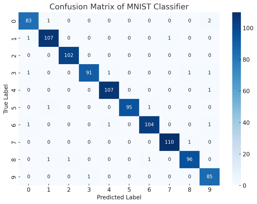
These metrics offer deeper insights into how well your model is performing beyond just raw accuracy.
Tips for Efficient Training
Here are some practical tips to make your training process smoother:
- Use GPU by calling
.to(device)wheredevice = torch.device("cuda" if torch.cuda.is_available() else "cpu") - Monitor validation accuracy to avoid overfitting
- Use
torchvision.utils.make_gridto visualize a batch of images - Save and load your dataset with
torch.saveandtorch.loadto avoid redownloading every time
Conclusion
Loading and processing the MNIST dataset in PyTorch is a foundational task that helps you get comfortable with the framework’s data handling utilities. From downloading and normalizing data to augmenting and feeding it into neural networks, every step contributes to building a robust machine learning pipeline.
Whether you’re just starting out or refining your PyTorch skills, mastering the MNIST workflow sets a solid foundation for tackling more complex datasets and tasks. With PyTorch’s rich ecosystem and tools like torchvision, you’ll find it straightforward to experiment and innovate.
Now that you understand the process of loading and processing the MNIST dataset in PyTorch, you’re ready to train models, tune hyperparameters, and dive deeper into deep learning!